Predicting Country of Origin
This project was an assignment for my machine learning class. We investigated data from the World Value Survey Version 7,
the survey includes participants from over 300 countries with over 250 questions ranging from religion to life satisfaction.
Our project was to use a random forest to determine variable importance and then create a logistic regression model to
predict country of origin from responses of citizens from the USA and Mexico. We were tasked with creating the
project in R and KNIME. Our file was provided in spss format.
Random Forest to Determine Variable Importance
Our first step is to narrow down the variables so our data is not so cluttered.
We want to use variables that are representative of beliefs, needs, values,
and attitudes to determine if the respondent resides in Mexico or US.
However, we need to be careful, as some variables are too specific.
i.e. Q223 asks the respondent to list country-specific political parties.
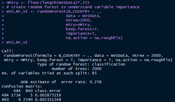
To narrow the variables down to a manageable level I used the randomForest
package in R to run 2,000 decision trees ranking variable importance in a descending order.
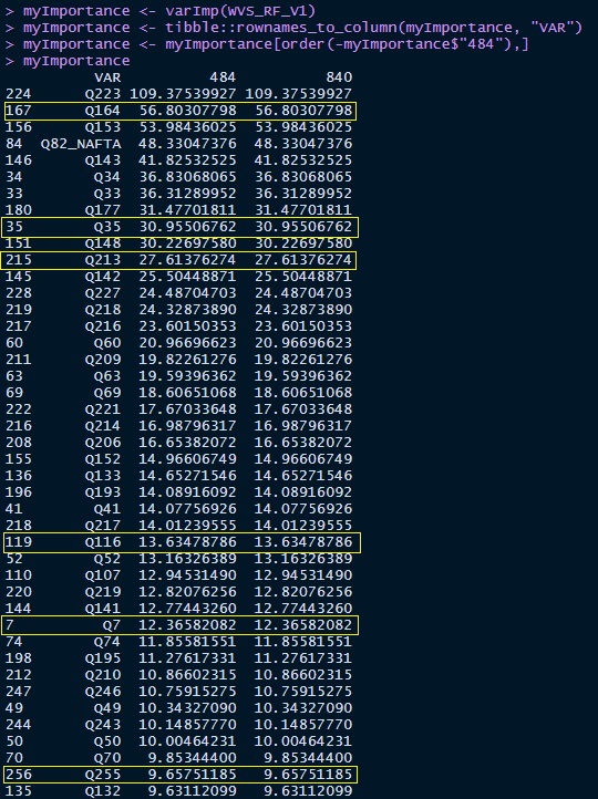
By limiting my search to variables with an importance greater than 9.5 the variables
were much more manageable. I referenced the World Value Survey and cultural atlases for
Mexico and US to better understand which variables would be representative of beliefs,
needs, values, and attitudes to pick my final variables. The variables chosen for the
logistic regression model are highlighted in yellow below:
Dependent and Independent Variables
B_COUNTRY is a nominal variable that specifies the respondent country of origin code.
The code for Mexico is ‘484’ and for USA is ‘840’. These two countries will be acting as my dependent variables.
The following survey questions were used as my independent variables:
- Q7 references encouraging children to learn good manners at home as being especially important.
- Q35 references the respondent’s agreement with the statement “if a woman earns more
money than her husband, it’s almost certain to cause problems.”
- Q116 references belief that civil service providers (police, judiciary, civil servants, doctors,
teachers) are involved in corruption.
- Q143 references the degree of worry the respondent has in not being able to give their children a good education.
- Q164 references the importance of God in the respondent’s life.
- Q213 references participating in political action and social activism by donating to a group or campaign.
- Q255 references how close the respondent feels to their village, town, or city.
Variable Validation and Transformations
To ensure that the variables were not Country specific I needed to look at the data,
some responses have Country code prefixes which would not be suitable for this model.
After looking at the data I looked at a summary of the variables:
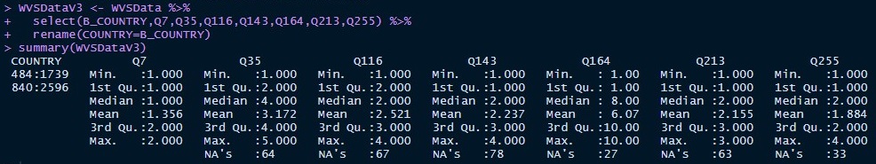
Verifying none of the variables were too Country specific I needed to deal with NA's.
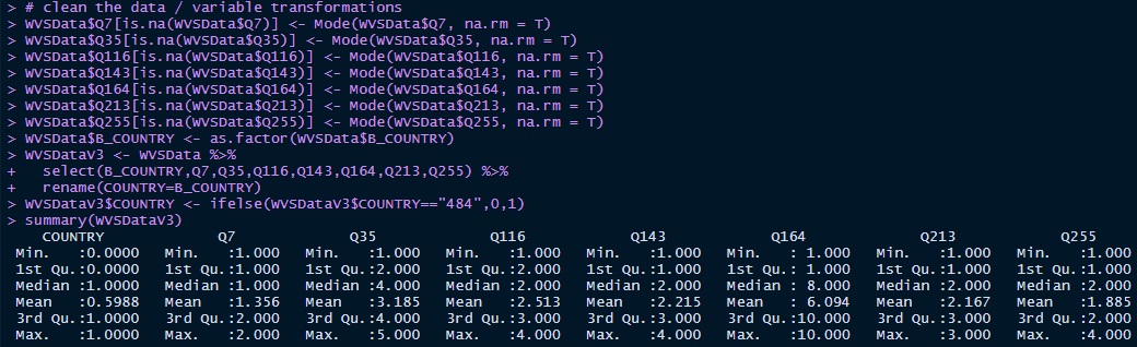
I decided to use mode imputation on the independent variables. Additionally I cast B_COUNTRY as a factor
and renamed B_COUNTRY to COUNTRY for ease of use. Finally I recoded Mexico to equal 0 and US to equal 1.
Now we can see there is no missingness:
Plotting Variables
Afterwards I plotted the variables by country to compare the distributions:
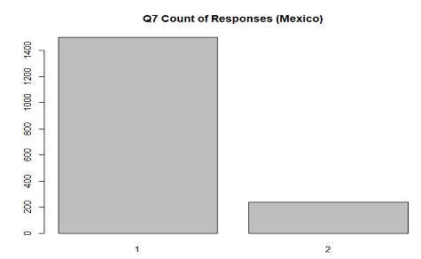
The distribution of responses in Mexico for Q7(child manners) where 1 is "Mentioned" and 2 is "Not mentioned"
With the importance of family and being a good host in Mexican culture this distribution makes sense.
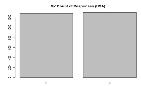
The distribution of responses in USA for Q7(child manners) where 1 is "Mentioned" and 2 is "Not mentioned"
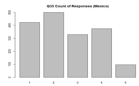
The distribution of responses in Mexico for Q35(high earning wife) where 1 is "Agree strongly" and 5 is
"Disagree strongly"
With strong traditional gender roles in Mexican families this distribution makes sense.
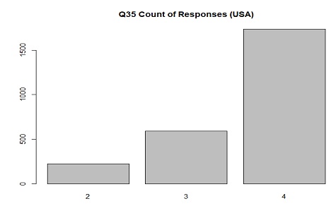
The distribution of responses in USA for Q35(high earning wife) where 1 is "Agree strongly" and 5 is
"Disagree strongly"
With weaker traditional gender roles in US families this distribution makes sense. Its interesting
that none of the respondents agreed or disagreed strongly.
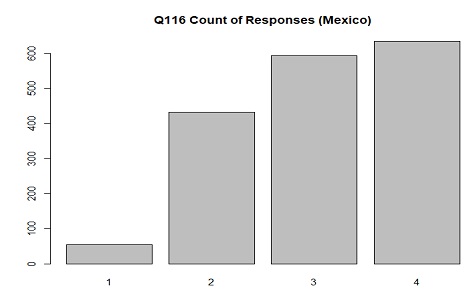
The distribution of responses in Mexico for Q116(civil service providers are corrupt) where 1 is
"None of them" and 4 is "All of them"
With the distrust in government overall in Mexico this distribution makes sense.
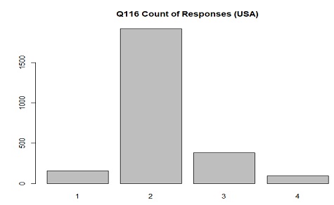
The distribution of responses in USA for Q116(civil service providers are corrupt) where 1 is
"None of them" and 4 is "All of them"
With US citizens having high trust in goverment overall this distribution makes sense.
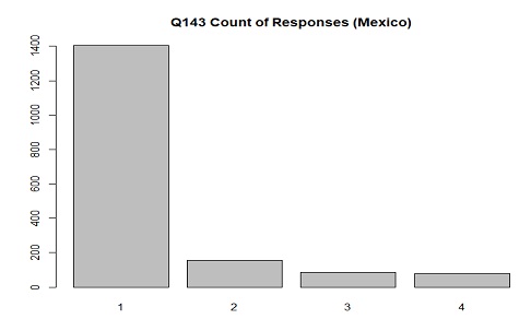
The distribution of responses in Mexico for Q143(worry about children's education) where 1 is "Very much" and
4 is "Not at all"
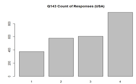
The distribution of responses in USA for Q143(worry about children's education) where 1 is "Very much" and
4 is "Not at all"
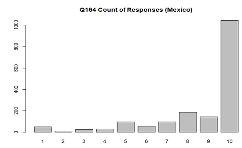
The distribution of responses in Mexico for Q164(importance of god) where 1 is "Not at all important" and 10 is "Very important"
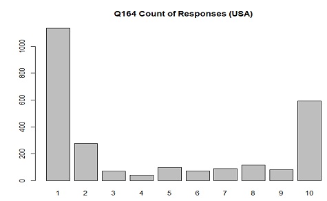
The distribution of responses in USA for Q164(importance of god) where 1 is "Not at all important" and 10 is "Very important"
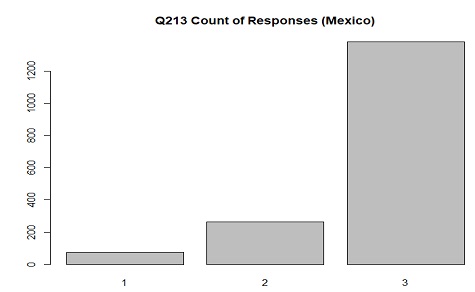
The distribution of responses in Mexico for Q213(action/activism through donating) where 1 is "Have done", 2 is "Might do",
and 3 is "Would never do"
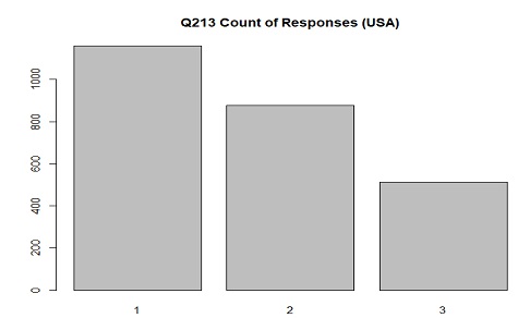
The distribution of responses in USA for Q213(action/activism through donating) where 1 is "Have done", 2 is "Might do",
and 3 is "Would never do"
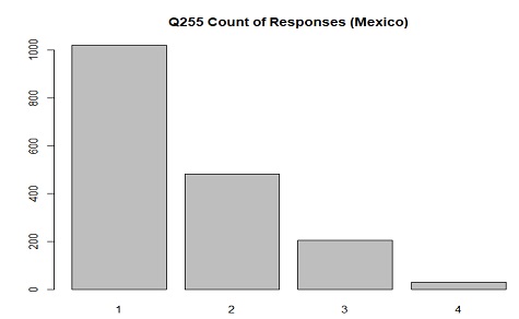
The distribution of responses in Mexico for Q255(closeness to village/town/city) where 1 is "Very close" and 4 is "Not close at all"
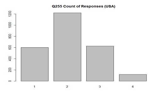
The distribution of responses in USA for Q255(closeness to village/town/city) where 1 is "Very close" and 4 is "Not close at all"
Logistic Regression Model
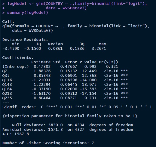
The summary below allows us to make an initial check of the model.
The first column we look at is the z value.
The further from 0 a value is, the stronger the variable is as a predictor.
In this case, we can see Q143(worry about children’s education) is the strongest predictor.
We also see that Q255(closeness to village/town/city) is our weakest predictor.
Looking at the p-value for all variables we see none are greater than 0.05 i.e. they are statistically significant.
Accuracy of Model
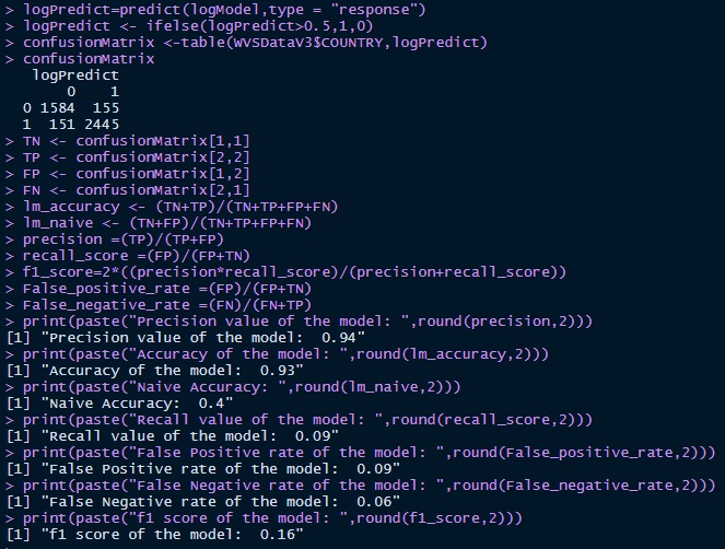
Finally we want to evaulate the accuracy of the model.
For this we look at the accuracy of the model compared to the naive model.
Additionally, we look at recall, false positive rate, false negative rate and the f1 score.
We can see that this model far outperforms the naive model with an accuracy of 93% compared to 40%
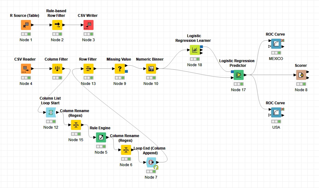
Repeat in KNIME
To demonstrate understanding of the concepts and adaptability, we were tasked with also creating the model in KNIME.
Because I am more comfortable in R and due to time constraints I did not recreate the random forest in KNIME to
determine variable importance, instead I just used the variables selected in R.
In KNIME I used the R Source node to load the spss file.
Then I narrow the dataset down to Mexico and US respondents with a row filter.
Then I saved the file as a CSV to ease of use in the KNIME model.
Using the scorer node we see that our model is producing a similar accuracy:

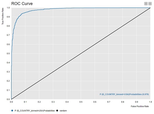
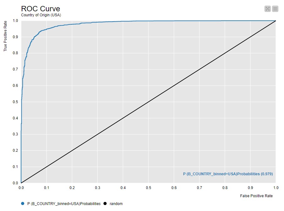
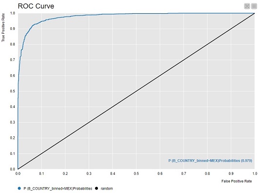
ROC Curves
Due to deadline constraints and ease of use I only created the ROC curves in KNIME.
In the future I would like to add the code to plot the ROC curves in R.
ROC Curve for Mexico:
ROC Curve for USA: